Navigation

Problem statement

System dynamics

Assuming zero slip of the trailer wheels, the nonlinear kinematics of a ground vehicle, shown in the following figure

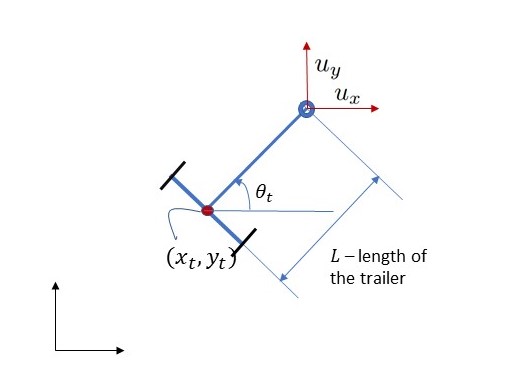
is given by the following equations

\[\begin{split} \dot{x}(t) {}={}& u_x(t) + L \sin \theta(t) \dot{\theta}(t)\\ \dot{y}(t) {}={}& u_y(t) - L \cos \theta(t) \dot{\theta}(t)\\ \dot{\theta}(t) {}={}& \tfrac{1}{L}(u_y(t) \cos \theta(t) - u_x(t) \sin \theta(t)) \end{split}\]

where the state vector $z=(x, y, \theta)$ comprises the coordinates $x$ and $y$ of the trailer and the heading angle $\theta$.

The input $u=(u_x, u_y)$ is a velocity reference which is tracked by a low-level controller.

The distance between the center of mass of the trailer and the fulcrum connecting to the towing vehicle is $L = 0.5\mathrm{m}$.

The system dynamics can be written concisely as

\[\dot{z}(t) = f(z(t), u(t)).\]

We shall discretise this system using the Euler discretization with sampling time $t_s$, that is

\[z_{t+1} = z_t + t_sf(z_{t}, u_{t}).\]

Cost functions

Our aim is to determine a sequence of control actions,

\[u = (u_0, u_1, \ldots, u_{N-1}),\]

so as to create a sequence of states $z_0,\ldots, z_N$, which reach as close as possible to a given target point $(x^{\mathrm{ref}}, y^{\mathrm{ref}})$ and a reference heading $\theta^{\mathrm{ref}}$.

To this end, we define the following stage cost function

\[\ell(z, u) = q [(x-x^{\mathrm{ref}})^2 + (y-y^{\mathrm{ref}})^2] + q_{\theta}(\theta-\theta^{\mathrm{ref}})^2 + r\|u\|^2,\]

where $q$, $q_\theta$ and $r$ are nonnegative weight coefficients.

Likewise, we define the terminal cost function

\[\ell_N(z) = q_N [(x-x^{\mathrm{ref}})^2 + (y-y^{\mathrm{ref}})^2] + q_{\theta,N}(\theta-\theta^{\mathrm{ref}})^2,\]

We now introduce the total cost function

\[V(u; z_0) = \sum_{t=0}^{N-1}\ell(z_t, u_t) + \ell_N(z_N),\]

where the sequence of states, $z_0,\ldots, z_N$ is governed by the discrete-time dynamics stated above.

Optimal control problem

We formulate the following optimal control problem

\[\begin{split}\operatorname*{Minimize}_{u {}\in{} \mathbb{R}^{2N}}&\ \ V(u; z_0)\\ \mathrm{subject\ to} &\ \ u \in U(z_0)\end{split}\tag{4}\]

We assume there are no active constraints on the input variables, that is $U(z_0) = \mathbb{R}^{2N}$.

Note that the sequence of states, $z_0, z_1, \ldots, z_N$, does not partipate in the problem definition in (4). This is because $z_t = z_t(z_0, u_0, \ldots, u_{t-1})$ for all $t=1,\ldots, N$. In order words, all $z_t$ are functions of $u$ and $z_0$.

Code generation in MATLAB

Firstly, we define the total cost function

% parameters
L = 0.5; ts = 0.1;

% Prediction horizon
N = 50; 

% target point and bearing
xref=1; yref=1; thetaref = 0;

% weights
q = 10; qtheta = .1; r = 1;
qN = 10*q; qthetaN = 10*qtheta;

nu = 2; nx = 3;
u = casadi.SX.sym('u', nu*N); 
z0 = casadi.SX.sym('z0', nx);

x = z0(1); y = z0(2); theta = z0(3);
cost = 0;
for t = 1:nu:nu*N
    cost = cost + q*((x-xref)^2 + (y-yref)^2) + qtheta*(theta-thetaref)^2;
    u_t = u(t:t+1);
    theta_dot = (1/L)*(u_t(2)*cos(theta) - u_t(1)*sin(theta));
    cost = cost + r*(u_t'*u_t);
    x = x + ts * (u_t(1) + L * sin(theta) * theta_dot);
    y = y + ts * (u_t(2) - L * cos(theta) * theta_dot);
    theta = theta + ts * theta_dot;
end
cost = cost + qN*((x-xref)^2 + (y-yref)^2) + qthetaN*(theta-thetaref)^2;

constraints = OpEnConstraints.make_no_constraints();

We then build the parametric optimizer:

builder = OpEnOptimizerBuilder()...
    .with_problem(u, z0, cost, constraints)...
    .with_build_name('navigation')...
    .with_build_mode('release')...
    .with_fpr_tolerance(1e-4)...
    .with_max_iterations(500);
optimizer = builder.build();

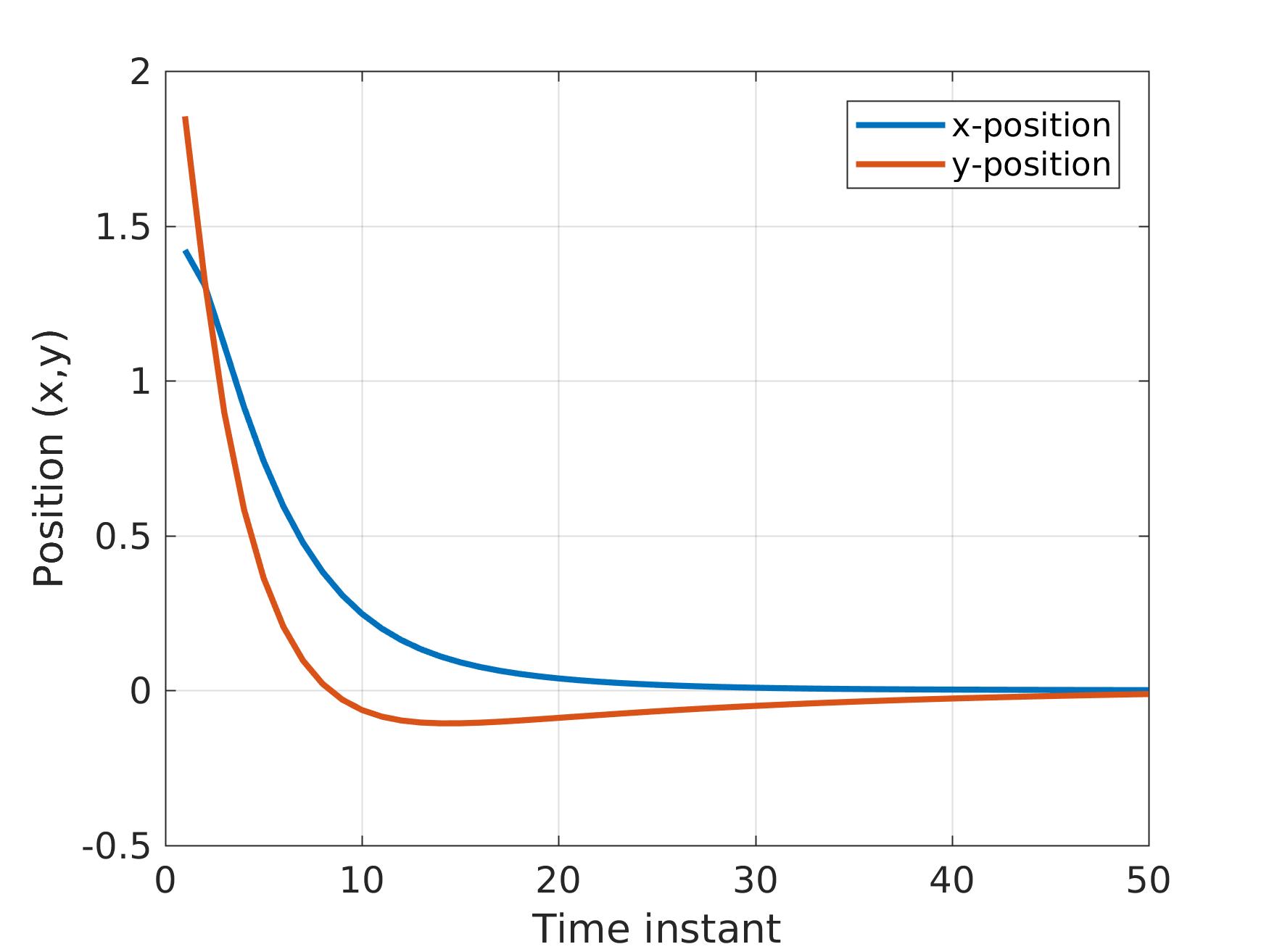
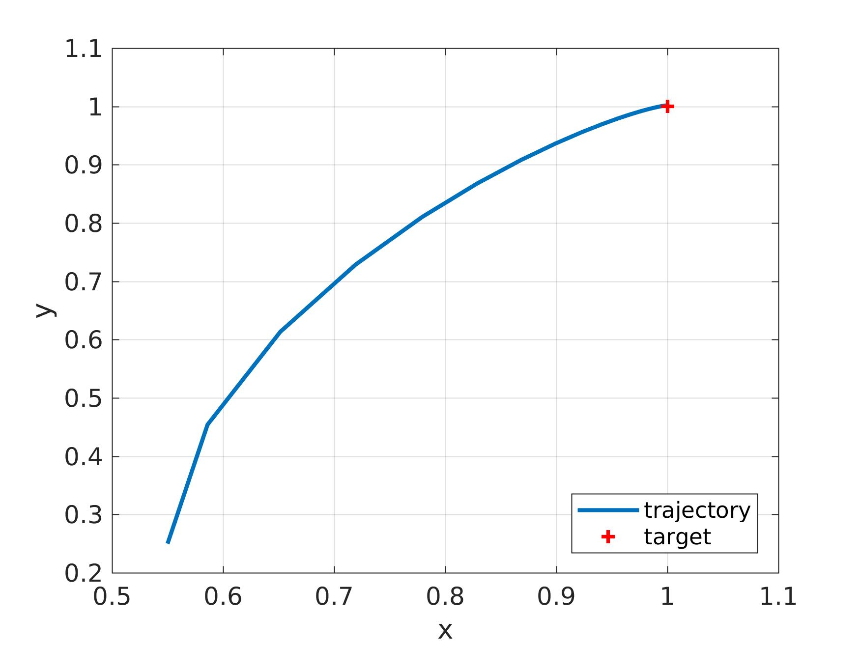
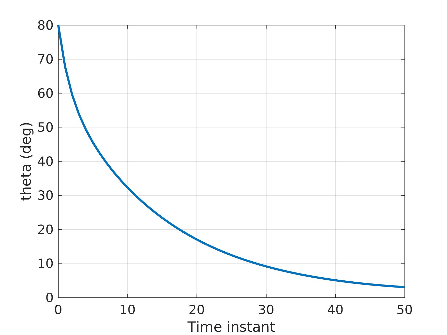
Solution

The solution is presented below (the algorithm converges in 25 iterations after 3.2ms):

Free references

Let's get a little creative!

We may define the parameter of the optimization problem to be

\[p = (z_0, z^{\mathrm{ref}})\]

where $z^{\mathrm{ref}} = (x^{\mathrm{ref}},y^{\mathrm{ref}},\theta^{\mathrm{ref}})$. This way, we will have an optimal control module that will allow us to plan trajectories from any initial position and pose to any final position and pose. This can then be used as a model predictive controller, where the references can be provided either by the user, manually, or by a higher-level system.

We will define the parameter $p$, instead of $z_0$, as follows:

p = casadi.SX.sym('p', 2*nx);
x = p(1); y = p(2); theta = p(3);
xref = p(4); yref = p(5); thetaref = p(6);

the rest of the problem definition remains the same.

The optimizer should now be called as follows:

z_init = [1.0; -0.3; deg2rad(30)];
z_ref  = [1.5;  0.7; deg2rad(50)];
out = optimizer.consume([z_init; z_ref]);

Obstacle avoidance

Consider the problem of determining a minimum-cost trajectory which avoids an obstacle, $O$, which is described by

\[O = \{z = (x,y) {}\mid{} h(z) > 0\},\]

where $h:\mathbb{R}^2\to\mathbb{R}$ is a $C^{1,1}$-function. The obstacle avoidance constraint $z\notin O$ is satisfied if and only if

\[[{}h(z){}]_+^2 {}={} 0,\]

where $[x]_+ = \max\{0, x\}$ is the plus operator.

We now define the modified stage cost function

\[\tilde{\ell}(z,u) {}={} \ell(z,u) + \eta [{}h(z){}]_+^2,\]

and the modified terminal cost function

\[\tilde{\ell}_N(z) {}={} \ell_N(z) + \eta_N [{}h(z){}]_+^2,\]

where $\eta$ and $\eta_N$ are positive weights. In the following plot we show trajectories for different values of $\eta$ and $\eta_N$...

For completeness, here is the modified code:

nu = 2; nx = 3;
u = casadi.SX.sym('u', nu*N); 
p = casadi.SX.sym('p', 2*nx+1);
x = p(1); y = p(2); theta = p(3);
xref = p(4); yref = p(5); thetaref=p(6);
h_penalty = p(end);
cost = 0;

% Obstacle (disc centered at `zobs` with radius `c`)
c = 0.4; zobs = [0.7; 0.5];

for t = 1:nu:nu*N
    z = [x; y];
    cost = cost + q*norm(z-zref) + qtheta*(theta-thetaref)^2;
    cost = cost + h_penalty * max(c^2 - norm(z-zobs)^2, 0)^2;
    u_t = u(t:t+1);
    theta_dot = (1/L)*(u_t(2)*cos(theta) - u_t(1)*sin(theta));
    cost = cost + r*(u_t'*u_t);
    x = x + ts * (u_t(1) + L * sin(theta) * theta_dot);
    y = y + ts * (u_t(2) - L * cos(theta) * theta_dot);
    theta = theta + ts * theta_dot;
end
cost = cost + qN*((x-xref)^2 + (y-yref)^2) + qthetaN*(theta-thetaref)^2;
cost = cost + h_penalty * max(c^2 - norm(z-zobs)^2, 0)^2;

Experimental validation

A somewhat more involved nonlinear model predictive control (NMPC) formulation, enhanced with obstacle avoidance capabilities, was presented in ECC '18.

A short footage of our experiment is shown below: