Getting started
The functionality presented here was introduced in opengen version 0.10.0a1. The API is still young and is likely to change in version 0.11.
OpEn now comes with a new module that facilitates the construction of optimal control problems. In an intuitive and straightforward way, the user defines the problem ingredients: stage costs, terminal costs, state and input constraints, and dynamics.
![]()
In a nutshell: quick overview
Suppose you want to solve the optimal control problem:
Suppose the state is two-dimensional and the input is one-dimensional. The dynamics is:
Here, a is a parameter. Suppose the stage cost function is:
Here, \(x^{\text{ref}}\), $q$, and $r$ are parameters. The terminal cost function is:
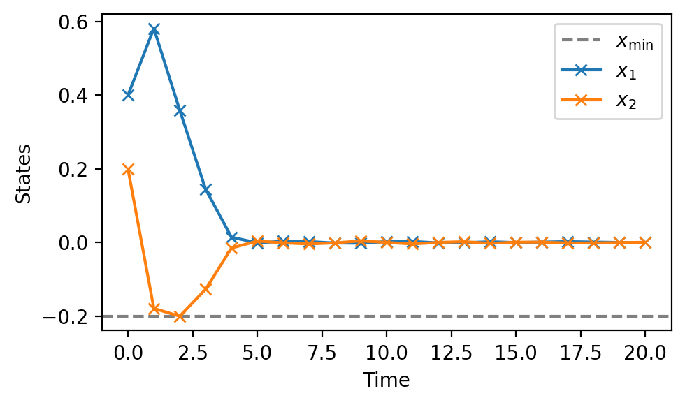
Lastly, we have the state constraint \(x_t \geq x_{\min}\), where \(x_{\min}\) is a parameter, and the hard input constraints \(\Vert u_t \Vert \leq 0.2\).
This optimal control problem can be constructed as follows:
![]()
import opengen as og
import casadi.casadi as cs
import numpy as np
import matplotlib.pyplot as plt

optimizer_name = "ocp_alm"

# Construct the OCP
ocp = og.ocp.OptimalControlProblem(nx=2, nu=1, horizon=20)

# Define the parameters
ocp.add_parameter("x0", 2)
ocp.add_parameter("xref", 2, default=[0.0, 0.0])
ocp.add_parameter("q", 1, default=1)
ocp.add_parameter("r", 1, default=0.1)
ocp.add_parameter("a", 1, default=0.8)
ocp.add_parameter("xmin", 1, default=-1)

# System dynamics
ocp.with_dynamics(lambda x, u, param:
                  cs.vertcat(0.98 * cs.sin(x[0]) + x[1],
                             0.1 * x[0]**2 - 0.5 * x[0] + param["a"] * x[1] + u[0]))
# Stage cost
ocp.with_stage_cost(
    lambda x, u, param, _t:
    param["q"] * cs.dot(x - param["xref"], x - param["xref"])
    + param["r"] * cs.dot(u, u)
)

# Terminal cost
ocp.with_terminal_cost(
    lambda x, param: 100 * cs.dot(x - param["xref"], x - param["xref"])
)

# State constraint: x1 <= xmax, imposed with ALM
ocp.with_path_constraint(
    lambda x, u, param, _t: x[1] - param["xmin"],
    kind="alm",
    set_c=og.constraints.Rectangle([0.], [np.inf]),
)

# Input constraints
ocp.with_input_constraints(og.constraints.BallInf(radius=0.2))
Having defined the above OCP, we can build the optimizer...
![]()
- Direct interface
- TCP socket interface
ocp_optimizer = og.ocp.OCPBuilder(
    ocp,
    metadata=og.config.OptimizerMeta().with_optimizer_name(optimizer_name),
    build_configuration=og.config.BuildConfiguration()
        .with_build_python_bindings().with_rebuild(True),
    solver_configuration=og.config.SolverConfiguration()
        .with_tolerance(1e-5)
        .with_delta_tolerance(1e-5)
        .with_preconditioning(True)
        .with_penalty_weight_update_factor(1.8)
        .with_max_inner_iterations(2000)
        .with_max_outer_iterations(40),
).build()
ocp_optimizer = og.ocp.OCPBuilder(
    ocp,
    metadata=og.config.OptimizerMeta().with_optimizer_name(optimizer_name),
    build_configuration=og.config.BuildConfiguration()
        .with_tcp_interface_config(
            tcp_interface_config=og.config.TcpServerConfiguration(bind_port=3391)
        ).with_rebuild(True),
    solver_configuration=og.config.SolverConfiguration()
        .with_tolerance(1e-5)
        .with_delta_tolerance(1e-5)
        .with_preconditioning(True)
        .with_penalty_weight_update_factor(1.8)
        .with_max_inner_iterations(2000)
        .with_max_outer_iterations(40),
).build()
The optimizer can then be called as follows:
result = ocp_optimizer.solve(x0=[0.4, 0.2], q=30, r=1, xmin=-0.2)
and note that all parameters except x0 are optional; if not specified,
their default values will be used (the defaults were set when we constructed the
OCP). We can now plot the optimal sequence of inputs (result.inputs)
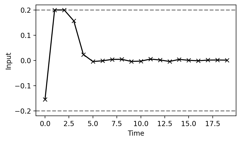
and the corresponding sequence of states (result.states)
The object result contains the above sequences of inputs and states and additional
information about the solution, solver time, Lagrange multipliers, etc.