Algorithm
Optimization Engine (OpEn) solves problems of the following form:
Our blanket assumptions are:
A1. Function $f({}\cdot{}, p):\mathbb{R}^{n_u}\to\mathbb{R}$ is continuously differentiable in $u$ with $L$-Lipschitz gradient (which may depend on $p$)
A2. $U\subseteq \mathbb{R}^n$ is a nonempty set on which we can compute projections (e.g., boxes, balls, discrete sets, etc); this set may possibly be nonconvex
A3. Mapping $F_1({}\cdot{}, p):\mathbb{R}^n\to\mathbb{R}^{n_1}$ has partial derivatives and $C$ is a closed, convex set from which we may compute distances, that is,
A4. Mapping $F_2({}\cdot{}, p):\mathbb{R}^n\to\mathbb{R}^{n_2}$ has partial derivatives
Simple constraints
Let us first focus on problems of the following simpler form (we have dropped the dependence on $p$ for the sake of brevity)
Projected gradient method
Recall that the projected gradient method applied on this problem yields the iterations
starting from an initial guess $u^0$.
Let us define $T_\gamma(u) = \Pi_U (u - \gamma \nabla f(u))$, so the projected gradient method can be written as $u^{\nu+1} = T_\gamma(u^\nu)$, that is, they satisfy
We call such points $u^\star$, $\gamma$-critical points of the problem.
If $\gamma < 2/L$, then the projected gradient method is guaranteed to converge in the sense that all accumulation points of the projected gradient method are fixed points of $T_\gamma$.
The projected gradient method involves only simple steps which makes it easy to program and suitable for embedded applications, but convergence is at most Q-linear, often slow and sensitive to ill conditioning.
Speeding things up
In order to achieve superior congerence rates we proceed as follows: a $\gamma$-crtical point of the above problem is a zero of the residual operator
We may, therefore, use a Newton-type method of the form
where $d^\nu$ is computed as
where $H_\nu$ are invertible linear operators that satisfy the secant condition $s^\nu = H_\nu y^\nu$ with $s^\nu = u^{\nu+1}-u^\nu$ and $y^\nu = R_\gamma(u^{\nu+1})-R_\gamma(u^{\nu})$.
We could then use fast L-BFGS quasi-Newtonian directions, which do not require matrix operations (only vector products) and have low memory requirements. However, convergence is only local, in a neighbourhood of a critical point $u^\star$.
Our objective is to employ a globalisation technique using an appropriate exact merit function.
Forward-Backward Envelope
The forward-backward envelope (FBE) is a function $\varphi_\gamma:\mathbb{R}^n\to\mathbb{R}$ is a function with the following properties
- It is real-valued
- It is continuous
- For $0 < \gamma < \tfrac{1}{L}$ it shares the same local/strong minima with the original problem
Therefore, the original constrained optimisation problem is equivalent to the unconstrained minimisation problem of function $\varphi_\gamma$.
Additionally, if $f\in C^2$, then FBE is $C^1$ with gradient $\nabla \varphi_\gamma(u) = (I-\gamma \nabla^2 f(u))R_\gamma(u)$.
The FBE is constructed as follows: Function $f$ can be approximated at a point $u \in U$ by the (local) quadratic upper bound:
Then, the FBE is defined as
This construction is illustrated in the figure below
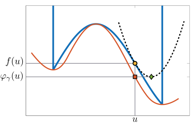
Provided that it is easy to compute the distance to $U$, the FBE can be easily computed by
PANOC
The proximal averaged Newton-type method (PANOC) takes averaged iterated that combine safe projected gradient updates and fast quasi-Newtonian directions, that is
and $\tau_\nu$ is chosen so that
for an appropriately chosen positive constant $\sigma$. You mean find more information about the algorithm in this paper.
Some facts about PANOC:
- It uses the same oracle as the projected gradient method
- Eventually only fast updates are activated: $u^{\nu+1} = u^\nu + d^\nu$
- The sequence $r^\nu$ goes to 0 sq. summably
- The cluster points of $u^\nu$ and $\bar{u}^\nu$ are $\gamma$-critical points
- No need to solve any linear systems
- Converges globally
- and it is very fast in practice
General constraints
Penalty Method
Let us now move on to problems with more general constraints of the general form
Equality constraints of the form $F_2(u) = 0$ can be used to accommodate inequality ones of the form
by taking $F_2(u) = \max\{0, h(u)\}$. Similarly, constraints of the form
where $\Phi:\mathbb{R}^{n_u}\to\mathbb{R}^{n_2}$ and $A\subseteq\mathbb{R}^{n_2}$, can be encoded by $F_2(u) = \operatorname{dist}_A(\Phi(u))$.
Although PANOC cannot solve the above problem directly, it can solve the following relaxed problem
Starting from an initial $\lambda_0 > 1$, we solve $\mathbb{P}(\lambda_\nu)$, we update $\lambda_{\nu+1} = \rho \lambda_{\nu}$, for some $\rho > 1$, and we then solve $\mathbb{P}(\lambda_{\nu+1})$ using the previous optimal solution, $u_\nu^\star$, as an initial guess. We call $\rho$ the penalty update coefficient.
This procedure stops once $\|F_2(u^\nu)\|_\infty {}<{} \delta$ for some tolerance $\delta > 0$. Tolerance $\delta$ controls the infeasibility of the solution.
Typically, few such outer iterations are required to achive a reasonable satisfaction of the constraints, while inner problems are solved very fast using PANOC.
Augmented Lagrangian Method
Similar to the penalty method, the augmented Lagrangian method (ALM) is used to solve constrained optimization problems by performing an "outer" iterative procedure, at every iteration of which, we need to solve an "inner" optimization problem. ALM updates both a penalty parameter as well as a vector $y$, known as the vector of Lagrange multipliers.
The inner optimization problems have the following form
where
This problem can be solved using PANOC.
At every outer iteration, $\nu$, the vector of Lagrange multipliers is updated according to
where $u^{\nu}$ is an (approximate) solution of the inner problem, $\mathbb{P}(p, c_{\nu}, y^{\nu})$, which is obtained using PANOC.
Inputs: $\epsilon, \delta > 0$ (tolerance), $\nu_{\max}$ (maximum number of iterations), $c_0 > 0$ (initial penalty parameter), $\epsilon_0 > \epsilon$ (initial tolerance), $\rho > 1$ (update factor for the penalty parameter), $\beta \in (0, 1)$ (decrease factor for the inner tolerance), $\theta \in (0, 1)$ (sufficient decrease coefficient), $u^0 \in \mathbb{R}^n$ (initial guess), $y^0 \in \mathbb{R}^{n_1}$ (initial guess for the Lagrange multipliers), $Y \subseteq \mathrm{dom}\ \delta_C^*$ (compact set)
Procedure: The ALM/PM algorithm performs the following iterations:
- $\bar{\epsilon} = \epsilon_0$, $y\gets{}y^0$, $u\gets{}u^0$, $t,z\gets{}0$
- For $\nu=0,\ldots, \nu_{\max}$
- $y \gets \Pi_Y(y)$
- $u \gets \arg\min_{u\in U} \psi(u, \xi)$, where $\psi(u, \xi)$ is a given function: this problem solved with tolerance $\bar\epsilon$
- $y^+ \gets y + c(F_1(u) - \Pi_C(F_1(u) + y/c))$
- Define $z^+ \gets \Vert y^+ - y \Vert$ and $t^+ = \Vert F_2(u) \Vert$
- If $z^+ \leq c\delta$, $t^+ \leq \delta$ and $\epsilon_\nu \leq \epsilon$, return $(u, y^+)$
- else if not ($\nu=0$ or ($z^+ \leq \theta z$ and $t^+ \leq \theta t$)), $c \gets \rho{}c$
- $\bar\epsilon \gets \max\{\epsilon, \beta\bar{\epsilon}\}$