Ball and Plate

Problem statement

Before we start

We will need to import the following libraries in Python:

import casadi.casadi as cs
import opengen as og
import matplotlib.pyplot as plt
import numpy as np

System dynamics

Consider the ball-and-beam system in the following figure

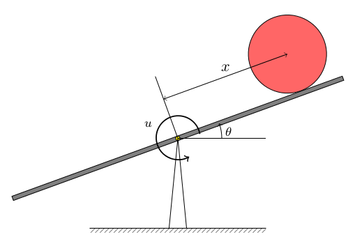
A ball of mass m is placed on a beam which is poised on a fulcrum at its middle. We can control the system by applying a torque $u$ with respect to the fulcrum point. The moment of inertia of the beam is denoted by $I$. The displacement $x$ of the ball from the midpoint can be measured with an optical sensor. The dynamical system is described by the following nonlinear differential equations

\[ \begin{align} \dot{x}_1 {}={}& x_2 \\ \dot{x}_2 {}={}& \tfrac{5}{7}(x_1x_4^2 - g\sin(x_3)) \\ \dot{x}_3 {}={}& x_4 \\ \dot{x}_4 {}={}& \frac{u - mgx_1\cos(x_3) - 2mx_1x_2x_3}{m x_1^2 + I} \end{align} \]

where $x_1=x$, $x_2=\dot{x}$, $x_3=\theta$ and $x_4 = \dot{\theta}$.

This is a continuous-time dynamical system of the form

\[ \dot{x} = f(x, u), \]

where $x=(x_1, x_2, x_3, x_4)$ is the system state and $u$ is the manipulated variable. The system parameters are

mass_ball = 1
moment_inertia = 0.0005
gravity_acceleration = 9.8044
sampling_time = 0.01
nx = 4
N = 15

and the continuous-time system dynamics is

def dynamics_ct(x, u):
    dx1 = x[1]
    dx2 = (5/7)*(x[0] * x[3]**2 - gravity_acceleration * cs.sin(x[2]))
    dx3 = x[3]
    dx4 = (u - mass_ball*gravity_acceleration*x[0]*cs.cos(x[2]) 
           - 2*mass_ball*x[0]*x[1]*x[3]) \
          / (mass_ball * x[0]**2 + moment_inertia)
    return [dx1, dx2, dx3, dx4]

We may discretize the system dynamics using, for example, the Euler discretization with sampling time $T_s$, that is, the discrete-time dynamics can be approximated by

\[ x_{t+1} = x_t + T_s f(x_t, u_t). \]

Let us write a little Python function for the discrete-time dynamics of the system

def dynamics_dt(x, u):
    dx = dynamics_ct(x, u)
    return [x[i] + sampling_time * dx[i] for i in range(nx)]

Nonlinear MPC problem

We shall construct a nonlinear MPC controller that drives the ball to the reference position $x_1^{\mathrm{ref}}=0$, i.e., at the reference state $x^{\mathrm{ref}}=(0,0,0,0)$ with input reference $u^{\mathrm{ref}}=0$.

To that end, let us define a state cost function $\ell(x, u)$ and a terminal cost function $\ell_N(x)$ as follows

\[ \begin{align} \ell(x, u) {}={}& \sum_{i=1}^{4}q_ix_i^2 + ru^2 \\ \ell_N(x) {}={}& \sum_{i=1}^{4}q_i^N x_i^2 \end{align} \]

In particular, let

def stage_cost(x, u):
    cost = 5*x[0]**2 + 0.01*x[1]**2 + 0.01*x[2]**2 + 0.05*x[3]**2 + 2.2*u**2
    return cost


def terminal_cost(x):
    cost = 100*x[0]**2 + 50*x[2]**2 + 20*x[1]**2 + 0.8*x[3]**2
    return cost

the cost parameters where selected arbitrarily.

The total cost function of the model predictive controller, along a prediction horizon $N$ will be

\[ V(x_0, u_0, \ldots, u_{N-1}) = \sum_{t=0}^{N-1}\ell(x_t, u_t) + \ell_N(x_N) \]

where $x_0$ is the given current state and $x_{t+1} = x_t + T_sf(x_t, u_t)$ as discussed above.

u_seq = cs.MX.sym("u", N)  # sequence of all u's
x0 = cs.MX.sym("x0", nx)   # initial state

x_t = x0
total_cost = 0
for t in range(0, N):
    total_cost += stage_cost(x_t, u_seq[t])  # update cost
    x_t = dynamics_dt(x_t, u_seq[t])         # update state

total_cost += terminal_cost(x_t)  # terminal cost

Lastly, we will impose the following input constraints

\[ -0.95 \leq u_t \leq 0.95 \]

for all $t=0,\ldots,N-1$. For that purpose, we shall define the following set

U = og.constraints.BallInf(None, 0.95)

Code generation

We may now specify the problem and generate code

problem = og.builder.Problem(u_seq, x0, total_cost)  \
            .with_constraints(U)

build_config = og.config.BuildConfiguration()  \
    .with_build_directory("python_build")      \
    .with_tcp_interface_config()

meta = og.config.OptimizerMeta().with_optimizer_name("ball_and_plate")

solver_config = og.config.SolverConfiguration()\
    .with_tolerance(1e-6)\
    .with_initial_tolerance(1e-6)

builder = og.builder.OpEnOptimizerBuilder(problem, meta,
                                          build_config, solver_config)
builder.build()

This will generate a solver in Rust as well as a TCP server that will listen for requests at localhost:8333 (this can be configured).

Simulations

Closed-loop trajectories

We can now easily call the auto-generated solver through its TCP socket in a few lines of code:

# Create a TCP connection manager
mng = og.tcp.OptimizerTcpManager("python_build/ball_and_plate")

# Start the TCP server
mng.start()

# Run simulations
x_state_0 = [0.1, -0.05, 0, 0.0]
simulation_steps = 2000

state_sequence = x_state_0
input_sequence = []

x = x_state_0
for k in range(simulation_steps):
    solver_status = mng.call(x)
    us = solver_status['solution']
    u = us[0]
    x_next = dynamics_dt(x, u)
    state_sequence += x_next
    input_sequence += [u]
    x = x_next

# Thanks TCP server; we won't be needing you any more
mng.kill()

We may now plot the closed-loop trajectories using matplotlib as follows

time = np.arange(0, sampling_time*simulation_steps, sampling_time)

plt.plot(time, state_sequence[0:4*simulation_steps:4], '-', label="position")
plt.plot(time, state_sequence[2:4*simulation_steps:4], '-', label="angle")
plt.grid()
plt.ylabel('states')
plt.xlabel('Time')
plt.legend(bbox_to_anchor=(0.7, 0.85), loc='upper left', borderaxespad=0.)
plt.show()

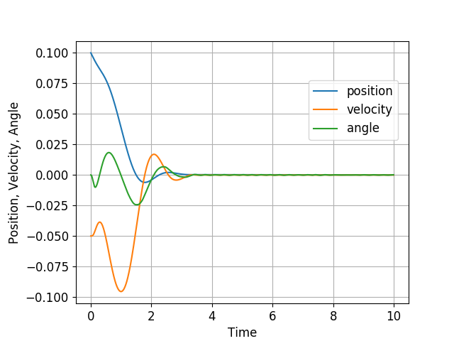
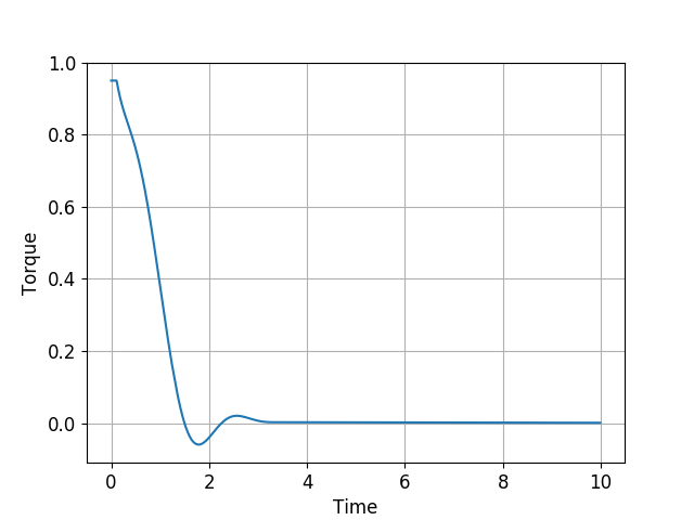
and a couple of plots from a different initial condition:

Solver statistics

In the above simulations, the average solution time is 0.35ms and the maximum time is 2.78ms.

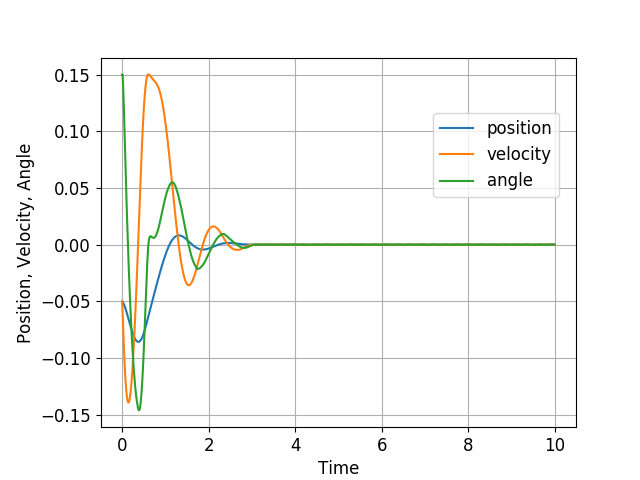
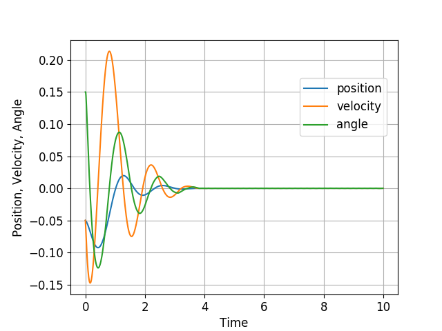
State constraints

In the second simulation scenario above, we see that the speed, $\dot{x}$, of the ball becomes larger than 0.2m/s. Let us impose the bound

\[ -0.15 \leq x_{2, t} \leq 0.15 \]

We may impose this constraint using the augmented Lagrangian method with the mapping $F_1$ and the set $C$ specified below:

x_t = x0
total_cost = 0
F1 = []
for t in range(0, N):
    total_cost += stage_cost(x_t, u_seq[t])  # update cost
    x_t = dynamics_dt(x_t, u_seq[t])         # update state
    F1 = cs.vertcat(F1, x_t[1])              # state constraint

C = og.constraints.BallInf(None, 0.15)    

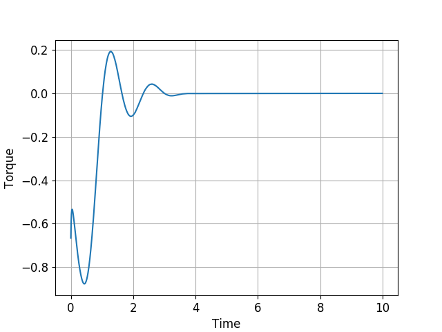
We then need to provide $F_1$ and $C$ to Problem as follows:

problem = og.builder.Problem(u_seq, x0, total_cost)  \
            .with_constraints(U)\
            .with_aug_lagrangian_constraints(F1, C)

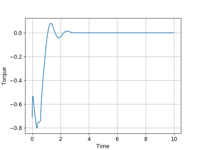
The system response is then shown below: