Nonlinear State Estimation

Problem statement

Consider a dynamical system, for simplicity, but without loss of generality without an actuation, with dynamics

\[ x_{t+1} = f(x_t) + w_t, \]

where $w_t$ is an unknown disturbance signal. We are able to measure the system's output through

\[ y_{t} = h(x_t) + v_t, \]

where $v_t$ is the measurement error.

Given a set of measurements $Y_N=(y_{0},\ldots,y_{N-1})$, our objective is to determine estimates $\hat{x}_t$ for all $t=0,\ldots,N$.

The estimation problem consists in solving the following optimization problem

\[ \begin{align} \operatorname*{Minimize}_{\hat{x}_0, \hat{\mathbf{w}}, \hat{\mathbf{v}}} & \sum_{t=0}^{N-1}\|\hat{w}_t\|^2_Q + \|\hat{v}_t\|^2_R \\ \text{subject to: }& \hat{x}_{t+1} = f(\hat{x}_t) + \hat{w}_t \\ & y_t = h(\hat{x}_t) + \hat{v}_t, t=0,\ldots, N-1. \end{align} \]

By eliminating all $\hat{w}_t$ and $\hat{v}_t$, the problem becomes

\[ \mathbb{P}(\mathbf{y}) {}:{} \operatorname*{Minimize}_{\hat{\mathbf{x}}} \sum_{t=0}^{N-1}\|\hat{x}_{t+1} - f(\hat{x}_t)\|^2_Q + \|y_t - h(\hat{x}_t)\|^2_R \]

The solution of this problem generates an optimal estimate

\[ \hat{\mathbf{x}}^\ast=(\hat{x}_0^*,\ldots,\hat{x}_{N}^*). \]

Such problems are used in moving horizon estimation with zero prior weighting.

Data Generation

Consider the Euler-discretization of the Lorenz system given by

\[ x_{t+1} = x_{t} + t_s \begin{bmatrix} \sigma (x_{2, t} - x_{1,t}) \\ x_{1, t} (\rho - x_{3, t}) - x_{2, t} \\ x_{1, t} x_{2, t} - \beta x_{3, t} \end{bmatrix} + w_t, \]

where $t_s$ is the sampling time, $\sigma$, $\rho$ and $\beta$ are constant parameters, $x_t = (x_{1, t}, x_{2, t}, x_{3, t})$ is the system state and $w_t$ is an unknown disturbance.

The measurements are obtained via the system output $y_t \in \mathbb{R}^3$ given by

\[ y_{t} = \begin{bmatrix} 2x_{1, t} \\ x_{2, t} + x_{3, t} \\ \tfrac{1}{10}x_{3, t}^2 - x_{1, t} \end{bmatrix} + v_t, \]

where $v_t\in\mathbb{R}^3$ in a measurement noise term.

Let us first generate output data from this system.

# Some necessary imports
# ------------------------------------
import opengen as og
import casadi.casadi as cs
import numpy as np
import matplotlib.pyplot as plt
from mpl_toolkits.mplot3d import Axes3D

# Generate data
# ------------------------------------
(rho, sigma, beta, ts) = (28.0, 10.0, 8.0/3.0, 0.02)
nx = ny = 3
Tsim = 100


def lorenz_sys(x):
    y = [sigma * (x[1] - x[0]),
         x[0] * (rho - x[2]) - x[1],
         x[0] * x[1] - beta * x[2]]
    return y


def dynamics(x):
    dx = lorenz_sys(x)
    return [x[idx] + ts*dx[idx] for idx in range(nx)]


def output(x):
    return [2.0*x[0], x[1]+x[2], x[2]**2/10.0-x[0]]

# Produce data
# ------------------------------------
x_data = [0.0] * (nx * Tsim)
y_data = [0.0] * (nx * Tsim)
x_data[0:nx] = [-10.0, -12.0, 27.0]
y_data[0:nx] = output(x_data[0:nx])

for i in range(Tsim-1):
    w = np.random.normal(0, 1, 3)
    v = np.random.normal(0, 1, 3)
    x_data[(i+1)*nx:(i+2)*nx] = dynamics(x_data[i*nx:(i+1)*nx]) + 0.02*w
    y_data[(i+1)*nx:(i+2)*nx] = output(x_data[(i+1)*nx:(i+2)*nx]) + 0.1*v

time = np.arange(0, ts*Tsim, ts)

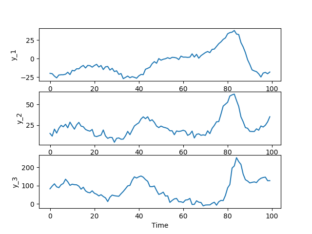
y_1 = y_data[0:ny*Tsim:ny]
y_2 = y_data[1:ny*Tsim:ny]
y_3 = y_data[2:ny*Tsim:ny]

plt.subplot(311)
plt.plot(time, y_1, '-')
plt.ylabel('y_1')
plt.subplot(312)
plt.plot(time, y_2, '-')
plt.ylabel('y_2')
plt.subplot(313)
plt.plot(time, y_3, '-')
plt.ylabel('y_3')
plt.xlabel('Time')
plt.show()

The output data are plotted below:

Code generation

def lorenz_sys_casadi(x):
    y = cs.vertcat(sigma * (x[1] - x[0]),
         x[0] * (rho - x[2]) - x[1],
         x[0] * x[1] - beta * x[2])
    return y


def dynamics_casadi(x):
    dx = lorenz_sys_casadi(x)
    return x + ts*dx


def output_casadi(x):
    return cs.vertcat(2.0*x[0], x[1]+x[2], x[2]**2/10.0-x[0])

# Problem definition
# ----------------------------------
X_hat = cs.SX.sym('Xhat', nx*(Tsim))
Y = cs.SX.sym('Y', nx*Tsim)
V = 0.0
print(X_hat)
for i in range(Tsim-1):
    w = X_hat[(i+1)*nx:(i+2)*nx] - dynamics_casadi(X_hat[i*nx:(i+1)*nx])
    v = Y[i*nx:(i+1)*nx] - output_casadi(X_hat[i*nx:(i+1)*nx])
    V += 20.0 * cs.dot(w, w) + 1.0 * cs.dot(v, v)

# Code generation
# ------------------------------------
problem = og.builder.Problem(X_hat, Y, V)
build_config = og.config.BuildConfiguration()  \
    .with_build_directory("my_optimizers") \
    .with_tcp_interface_config()
meta = og.config.OptimizerMeta()               \
    .with_optimizer_name("estimator")
builder = og.builder.OpEnOptimizerBuilder(problem, meta, build_config)
builder.build()

The generated solver can be consumed over its TCP interface:

# Use TCP server
# ------------------------------------
mng = og.tcp.OptimizerTcpManager('my_optimizers/estimator')
mng.start()

mng.ping()
solution = mng.call(y_data)
mng.kill()

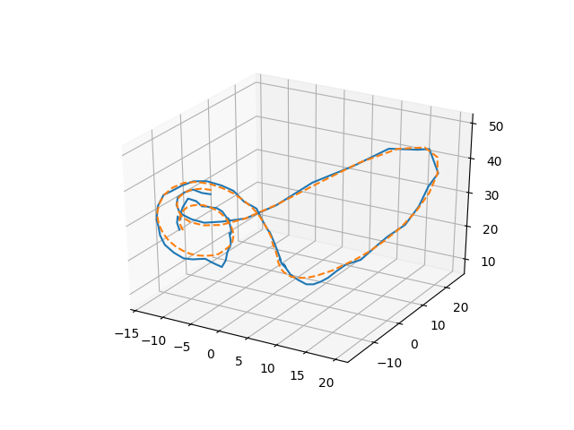
# Plot solution
x_star = solution['solution']
x_1_star = x_star[0:nx*Tsim:nx]
x_2_star = x_star[1:nx*Tsim:nx]
x_3_star = x_star[2:nx*Tsim:nx]
x_1 = x_data[0:nx*Tsim:nx]
x_2 = x_data[1:nx*Tsim:nx]
x_3 = x_data[2:nx*Tsim:nx]

fig = plt.figure()
ax = Axes3D(fig)
ax.plot(x_1_star,x_2_star,x_3_star)
ax.plot(x_1,x_2,x_3, '--')
plt.show()

This will generate a parametric optimizer for problem $\mathbb{P}(\mathbf{y})$ shown above that takes the system output, $\mathbf{y}$, and returns an estimate of the system state.

Such an estimation for the above randomly-generated data is shown below. The optimization problem was solved in 2.73 milliseconds (in 65 iterations).