Tandem tanks
Problem statement
Before we start
We will need to import the following libraries in Python:
import casadi.casadi as cs
import opengen as og
import matplotlib.pyplot as plt
import numpy as np
System dynamics
Consider the following system of tandem tanks
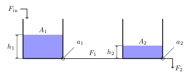
the tanks have cross-section areas $A_1$ and $A_2$, they store a liquid of density $\rho$ which can flow between the two tanks through a short pipe of cross-section area $a_1$. The liquid outflows from the second tank through an orifice of area $a_2$. The level of liquid in the two tanks, $h_1$ and $h_2$ is governed by the differential equations
so long as $h_1 > h_2$.
This is a continuous-time dynamical system of the form
a1 = 10*1e-4
a2 = 10*1.5e-4
A1 = 2.5
A2 = 0.1
rho = 998
g = 9.8044
sampling_time = 15
nx = 2
and the continuous-time system dynamics is
def dynamics_ct(x, u):
    h1 = x[0]
    h2 = x[1]
    dx1 = u/(rho * A1) - (a1 / A1) * cs.sqrt(2 * g * (h1 - h2))
    dx2 = (a1 * cs.sqrt(2 * g * (h1 - h2)) - a2 * cs.sqrt(h2))/A2
    return [dx1, dx2]
We may discretize the system dynamics using, for example, the Euler discretization with sampling time $T_s$, that is, the discrete-time dynamics can be approximated by
Let us write a little Python function for the discrete-time dynamics of the system
def dynamics_dt(x, u):
    dx = dynamics_ct(x, u)
    return [x[i] + sampling_time * dx[i] for i in range(nx)]
Nonlinear MPC problem
We shall construct a nonlinear MPC controller that drives the ball to the reference position $x_1^{\mathrm{ref}}=0$, i.e., at the reference state $x^{\mathrm{ref}}=(0,0,0,0)$ with input reference $u^{\mathrm{ref}}=0$.
To that end, let us define a state cost function $\ell(x, u)$ and a terminal cost function $\ell_N(x)$ as follows
In particular, let
q1 = 1
q2 = 1
qF = 0.5

qN1 = 50
qN2 = 50

def stage_cost(x, u):
    h1 = x[0]
    h2 = x[1]
    return q1 * (h1 - h1_ref)**2 + q2 * (h2 - h2_ref)**2 + qF * (u - F_ref)**2

def terminal_cost(x):
    h1 = x[0]
    h2 = x[1]
    return qN1 * (h1 - h1_ref)**2 + qN2 * (h2 - h2_ref)**2
The total cost function of the model predictive controller, along a prediction horizon $N$ will be
where $x_0$ is the given current state and $x_{t+1} = x_t + T_sf(x_t, u_t)$ as discussed above.
u_seq = cs.MX.sym("u", N)  # sequence of all u's
x0 = cs.MX.sym("x0", nx)   # initial state

x_t = x0
total_cost = 0
for t in range(0, N):
    total_cost += stage_cost(x_t, u_seq[t])  # update cost
    x_t = dynamics_dt(x_t, u_seq[t])         # update state

total_cost += terminal_cost(x_t)  # terminal cost
Lastly, we will impose the following input constraints
for all $t=0,\ldots,N-1$. For that purpose, we shall define the following set
U = og.constraints.Rectangle([8]*N, [11]*N)
Code generation
We may now specify the problem and generate code
problem = og.builder.Problem(u_seq, x0, total_cost)  \
            .with_constraints(U)

build_config = og.config.BuildConfiguration()  \
    .with_build_directory("python_build")      \
    .with_tcp_interface_config()

meta = og.config.OptimizerMeta().with_optimizer_name("ball_and_plate")

solver_config = og.config.SolverConfiguration()\
    .with_tolerance(1e-6)\
    .with_initial_tolerance(1e-6)

builder = og.builder.OpEnOptimizerBuilder(problem, meta,
                                          build_config, solver_config)
builder.build()
This will generate a solver in Rust as well as a TCP server that will
listen for requests at localhost:8333 (this can be configured).
Simulations
Closed-loop trajectories
We can now easily call the auto-generated solver through its TCP socket in a few lines of code:
# Create a TCP connection manager
mng = og.tcp.OptimizerTcpManager("python_build/ball_and_plate")

# Start the TCP server
mng.start()

# Run simulations
x_state_0 = [0.1, -0.05, 0, 0.0]
simulation_steps = 2000

state_sequence = x_state_0
input_sequence = []

x = x_state_0
initial_guess = None
for k in range(simulation_steps):
    solver_status = mng.call(x, initial_guess)
    us = solver_status['solution']
    u = us[0]
    initial_guess = us[1:] + [us[N-1]]
    x_next = dynamics_dt(x, u)
    state_sequence += x_next
    input_sequence += [u]
    x = x_next

# Thanks TCP server; we won't be needing you any more
mng.kill()
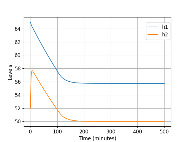
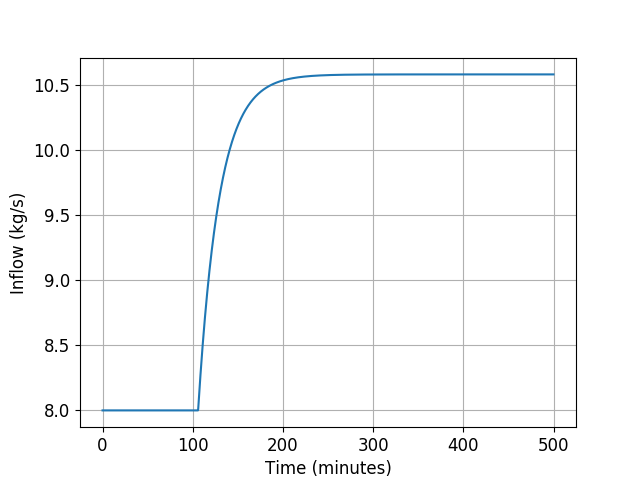
We may now plot the closed-loop trajectories using matplotlib as follows
time = np.arange(0, sampling_time*simulation_steps, sampling_time)

plt.plot(time, state_sequence[0:4*simulation_steps:4], '-', label="position")
plt.plot(time, state_sequence[2:4*simulation_steps:4], '-', label="angle")
plt.grid()
plt.ylabel('states')
plt.xlabel('Time')
plt.legend(bbox_to_anchor=(0.7, 0.85), loc='upper left', borderaxespad=0.)
plt.show()
Solver statistics
In the above simulations, the average solution time is 134us and the maximum time is 1.77ms. We ran a second set of simulations with double the original prediction horizon, namely $N=240$, and the average solution time increased to 343us and the maximum time was 1.44ms.