Navigation of ground vehicle

Unobstructed navigation

Consider the navigation problem for an autonomous ground vehicle which carries a trailer as illustrated in the following figure.

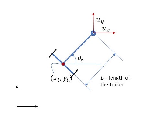
This is non-holonomic vehicle governed by the dynamical equations [Ref, Section IV]:

\[ \begin{align} \theta_{t+1} {}={}& \theta_t + t_s\tfrac{1}{L}(u_{y,t} \cos \theta_t - u_{x,t} \sin \theta_t), \\ x_{t+1} {}={}& x_t + t_s [u_x + \sin\theta_t(u_{y,t} \cos \theta_t - u_{x,t} \sin \theta_t)], \\ y_{t+1} {}={}& y_t - t_s [u_y + \cos\theta_t(u_{y,t} \cos \theta_t - u_{x,t} \sin \theta_t)]. \end{align} \]

We want to solve the following optimal control problem

\[ \begin{align} \mathbb{P}(p){}:{}\operatorname*{Minimize}_{u_0, \ldots, u_{N-1}}& \sum_{i=1}^{N - 1} \|z_t-z^{\mathrm{ref}}\|_Q^2 + r \|u_t\|^2 + \|z_N-z^{\mathrm{ref}}\|_{Q_N}^2 \\ \text{subject to: }& z_{t+1} = f(z_t, u_t), t=0,\ldots, N-1 \\ &u_{\min} \leq u_t \leq u_{\max}, t=0,\ldots, N-1 \\ &z_0=p \end{align} \]

where $z = (x,y,\theta)$ is the position and orientation of the vehicle, $z^{\mathrm{ref}}$ is the target position and orientation and $f$ describes the vehicle dynamics, which in this example is

\[ f(z, u) = \begin{bmatrix} x + t_s [u_x + \sin\theta (u_y \cos\theta - u_x \sin\theta) ] \\ y + t_s [u_y + \sin\theta (u_y \cos\theta - u_x \sin\theta) ] \\ \theta + t_s L^{-1} (u_y \cos\theta - u_x \sin\theta) \end{bmatrix} \]

import opengen as og
import casadi.casadi as cs
import matplotlib.pyplot as plt
import numpy as np

# Build parametric optimizer
# ------------------------------------
(nu, nx, N, L, ts) = (2, 3, 20, 0.5, 0.1)
(xref, yref, thetaref) = (1, 1, 0)
(q, qtheta, r, qN, qthetaN) = (10, 0.1, 1, 200, 2)

u = cs.SX.sym('u', nu*N)
z0 = cs.SX.sym('z0', nx)

(x, y, theta) = (z0[0], z0[1], z0[2])

cost = 0
for t in range(0, nu*N, nu):
    cost += q*((x-xref)**2 + (y-yref)**2) + qtheta*(theta-thetaref)**2
    u_t = u[t:t+2]
    theta_dot = (1/L) * (u_t[1] * cs.cos(theta) - u_t[0] * cs.sin(theta))
    cost += r * cs.dot(u_t, u_t)
    x += ts * (u_t[0] + L * cs.sin(theta) * theta_dot)
    y += ts * (u_t[1] - L * cs.cos(theta) * theta_dot)
    theta += ts * theta_dot

cost += qN*((x-xref)**2 + (y-yref)**2) + qthetaN*(theta-thetaref)**2

umin = [-3.0] * (nu*N)
umax = [3.0] * (nu*N)
bounds = og.constraints.Rectangle(umin, umax)

problem = og.builder.Problem(u, z0, cost).with_constraints(bounds)
build_config = og.config.BuildConfiguration()\
    .with_build_directory("my_optimizers")\
    .with_build_mode("debug")\
    .with_tcp_interface_config()
meta = og.config.OptimizerMeta()\
    .with_optimizer_name("navigation")
solver_config = og.config.SolverConfiguration()\
    .with_tolerance(1e-5)
builder = og.builder.OpEnOptimizerBuilder(problem,
                                          meta,
                                          build_config,
                                          solver_config)
builder.build()

We may now use the optimiser:

TCP Interface

Direct Interface

# Use TCP server
# ------------------------------------
mng = og.tcp.OptimizerTcpManager('my_optimizers/navigation')
mng.start()

mng.ping()
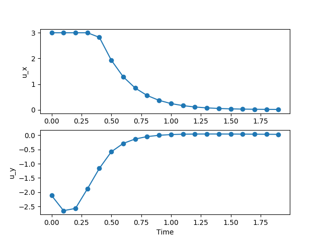
solution = mng.call([-1.0, 2.0, 0.0], initial_guess=[1.0] * (nu*N))
mng.kill()


# Plot solution
# ------------------------------------
time = np.arange(0, ts*N, ts)
u_star = solution['solution']
ux = u_star[0:nu*N:2]
uy = u_star[1:nu*N:2]

plt.subplot(211)
plt.plot(time, ux, '-o')
plt.ylabel('u_x')
plt.subplot(212)
plt.plot(time, uy, '-o')
plt.ylabel('u_y')
plt.xlabel('Time')
plt.show()

# Note: to use the direct interface you need to build using
#       .with_build_python_bindings()
import sys

# Use Direct Interface
# ------------------------------------
sys.path.insert(1, './my_optimizers/navigation')
import navigation

solver = navigation.solver()
result = solver.run(p=[-1.0, 2.0, 0.0],
                    initial_guess=[1.0] * (nu*N))
u_star = result.solution


# Plot solution
# ------------------------------------
time = np.arange(0, ts*N, ts)
ux = u_star[0:nu*N:2]
uy = u_star[1:nu*N:2]

plt.subplot(211)
plt.plot(time, ux, '-o')
plt.ylabel('u_x')
plt.subplot(212)
plt.plot(time, uy, '-o')
plt.ylabel('u_y')
plt.xlabel('Time')
plt.show()

This will produce the following plot:

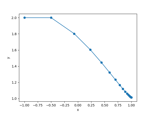
If you would like to plot the (x, y)-trajectories of the vehicle, run the following code:

# Plot trajectory
# ------------------------------------
x_states = [0.0] * (nx*(N+2))
x_states[0:nx+1] = x_init
for t in range(0, N):
    u_t = u_star[t*nu:(t+1)*nu]

    x = x_states[t * nx]
    y = x_states[t * nx + 1]
    theta = x_states[t * nx + 2]

    theta_dot = (1/L) * (u_t[1] * np.cos(theta) - u_t[0] * np.sin(theta))

    x_states[(t+1)*nx] = x + ts * (u_t[0] + L*np.sin(theta)*theta_dot)
    x_states[(t+1)*nx+1] = y + ts * (u_t[1] - L*np.cos(theta)*theta_dot)
    x_states[(t+1)*nx+2] = theta + ts*theta_dot

xx = x_states[0:nx*N:nx]
xy = x_states[1:nx*N:nx]

print(x_states)
print(xx)
plt.plot(xx, xy, '-o')
plt.show()

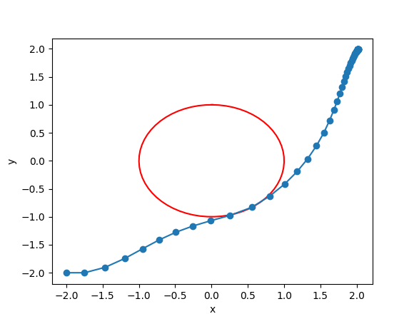
Obstructed navigation

Let us add an obstable: consider a ball centered at the origin with radius $r=1$, which needs to be avoided. To that end, we introduce the constraint $c(u; p) = 0$ where

\[c(u; p) = \sum_{t=0}^{N-1}[1-\|z_t\|^2]_+,\]

where $z_t=(x_t,y_t)$ is the position of the vehicle at time $t$ and $[z]_+ = \max\{0, z\}$.

The decision variable, as above, is $u = (u_0, \ldots, u_{N-1})$ and $z_t = z_t(u)$.

In order to define function $c$ in Python, we need to add one line in the above code:

c = 0
for t in range(0, N):
    cost += q*((x-xref)**2 + (y-yref)**2) + qtheta*(theta-thetaref)**2
    u_t = u[t*nu:(t+1)*nu]
    theta_dot = (1/L) * (u_t[1] * cs.cos(theta) - u_t[0] * cs.sin(theta))
    cost += r * cs.dot(u_t, u_t)
    x += ts * (u_t[0] + L * cs.sin(theta) * theta_dot)
    y += ts * (u_t[1] - L * cs.cos(theta) * theta_dot)
    theta += ts * theta_dot
    # ADD THIS LINE:
    c += cs.fmax(0, 1 - x**2 - y**2)

It makes sense to customize the solver parameters, especially the allowed violation of the constraints (with_delta_tolerance), the update factor for the penalty weights (with_penalty_weight_update_factor) and the initial weights (with_initial_penalty_weights):

solver_config = og.config.SolverConfiguration()\
    .with_tolerance(1e-4)\
    .with_initial_tolerance(1e-4)\
    .with_max_outer_iterations(5)\
    .with_delta_tolerance(1e-2)\
    .with_penalty_weight_update_factor(10.0)\
    .with_initial_penalty_weights(100.0)

Here is a trajectory of the system with $N=60$.

Update reference in real time

We may update the reference, $z^{\mathrm{ref}}$, in real time. If suffices to define $p = (z_0, z^{\mathrm{ref}})$. In other words, we use the parameter vector, $p$, to pass to the optimiser both the initial condition and the target.

We need to introduce the following changes. Firstly, we define the parameter vector:

p = cs.SX.sym('p', 2*nx)
(x, y, theta) = (p[0], p[1], p[2])
(xref, yref, thetaref) = (p[3], p[4], p[5])

and second update the problem definition to use p as the parameter vector:

problem = og.builder.Problem(u, p, cost).with_constraints(bounds)

Then, when we use the optimiser we to provide the vector p. For example, if z0 = (-1, 2, 0) and xref = 1, yref = 0.6, thetaref = 0.05 we use

result = solver.run(p=[-1.0, 2.0, 0.0, 1.0, 0.6, 0.05])